
From RF to Software
How a radio turns RF into I/Q samples, how one BPSK signal goes from bits to RF and back, and why that lets a ground station's modem run anywhere.
A satellite ground station was traditionally a room of dedicated boxes. Each carrier had its own hardware modem, wired to the antenna by cable. Those modems could be configured for many waveforms, but the processing lived inside dedicated equipment at the site. More and more of that room is now software. The antenna, the amplifiers and a digitizer stay at the site. The rest can run on a server somewhere else.
How does a radio wave become something a program can work on, and why can that program run anywhere? This post follows one signal from the antenna to bits and back to answer that. The running example is a 36 MHz Ku-band transponder, a common unit of satellite capacity.
The Carrier Is Huge, the Information Is Narrow
An antenna turns a radio wave into a voltage. That is all it does. On our Ku-band downlink the voltage swings about 12 billion times a second, but the information rides on slow changes in that swing. The transponder carries 36 MHz of content on a 12 GHz carrier.
Sampling the raw carrier would mean more than 24 billion samples a second to capture 36 MHz of content. So the receiver first moves the signal down to 0 Hz with a mixer, and only then samples it. Now the sample rate is set by the bandwidth of the content, about 40 million complex I/Q samples a second for the transponder (40 MS/s on each of the I and Q channels), not by the carrier.
Why Two Branches: I and Q
A sinusoid at a known frequency can change in two ways: its amplitude and its phase. Any signal near a carrier can be written as two slow waveforms riding on a cosine and a sine:
The cosine and sine are 90° apart, so they act as two independent axes. The receiver mixes the antenna voltage with each one and low-pass filters the result. The cosine branch gives and the sine branch gives . An analog-to-digital converter (ADC) on each branch then turns them into numbers, and each pair becomes one complex sample, .
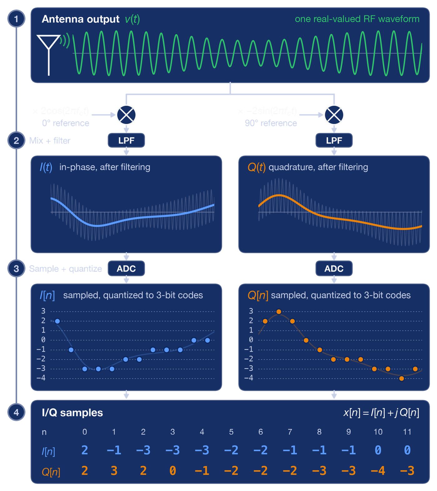
Why not one branch? With a single mixer, content just above the carrier and content just below it land on the same frequency after the shift, and the two can no longer be separated. With I and Q, content above the carrier becomes positive frequencies and content below becomes negative ones. Nothing is lost, and the sample rate only has to match the bandwidth.
Some radios sample earlier, at an intermediate frequency or even at RF, and do the mixing in software. The output is the same stream of I/Q samples. From here on, everything is arithmetic on those samples, starting with the modem.
Bits to RF and Back
A modem's job is to turn bits into I/Q samples on the way out and samples back into bits on the way in. A real one does that tens of millions of times a second. To see every step, this section uses a toy instead: nine bits, 101100101, small enough to follow one symbol at a time. They are sent with BPSK (one bit per symbol) through a root-raised-cosine filter with roll-off , the same roll-off as our transponder. The channel adds noise. Carrier and timing are assumed perfect. Every curve below comes from this one simulation.
Why Shape the Pulses
BPSK maps 1 to +1 and 0 to −1. Sent as is, that is a square wave, and sharp jumps spread energy far outside the signal's own band. On a shared transponder, that energy lands on the neighbours.
The transmitter smooths each symbol into a rounded pulse instead. In the figure, the smooth curve is the I component of the samples the software hands to the hardware. Q is zero: BPSK uses only one axis. A digital-to-analog converter and a mixer then put it on a carrier.
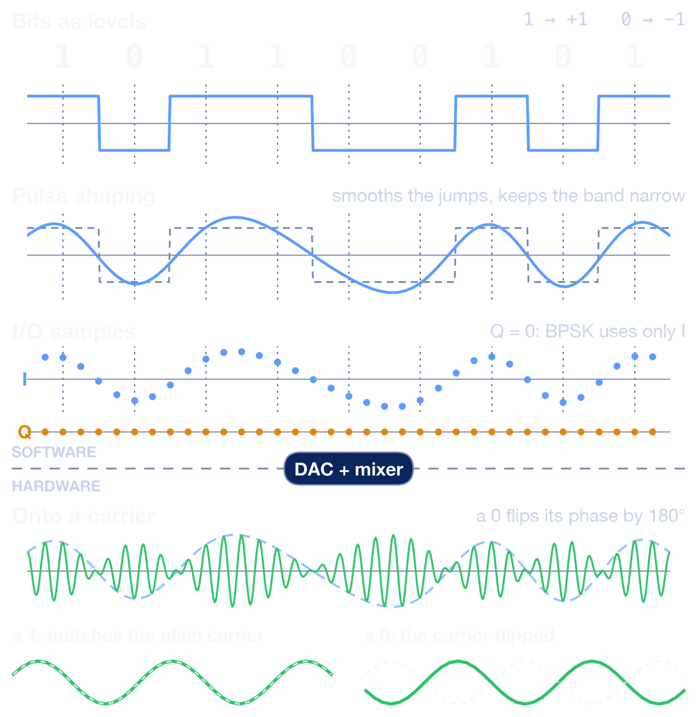
On the carrier, a positive I leaves the carrier in step with the reference and a negative I flips it by 180°. The bit is in that sign. The envelope dips where the sign changes, which can look like amplitude keying, but the carrier's strength carries no information. A 0 is the carrier flipped.
The payoff shows up in the spectrum.
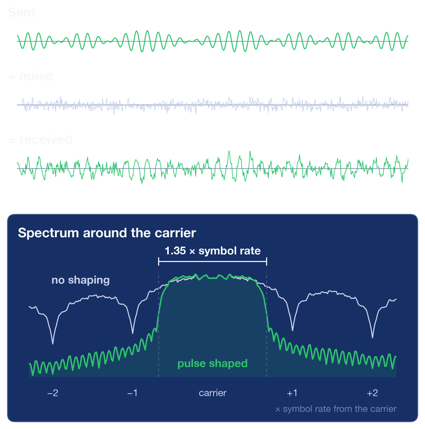
With shaping, the signal occupies
where is the symbol rate. Here that is 1.35 times the symbol rate. On our 36 MHz transponder, that means about 27 million symbols per second. The roll-off decides how much spectrum each symbol costs. At the 0.05 roll-off DVB-S2X allows, the same transponder carries about 34 million.
Why the Filter Is Split in Two
The receiver runs the chain backwards. The mixer and ADC turn the noisy RF into I/Q samples. Software applies a second root-raised-cosine filter, takes one sample at the centre of each symbol, and reads the sign.
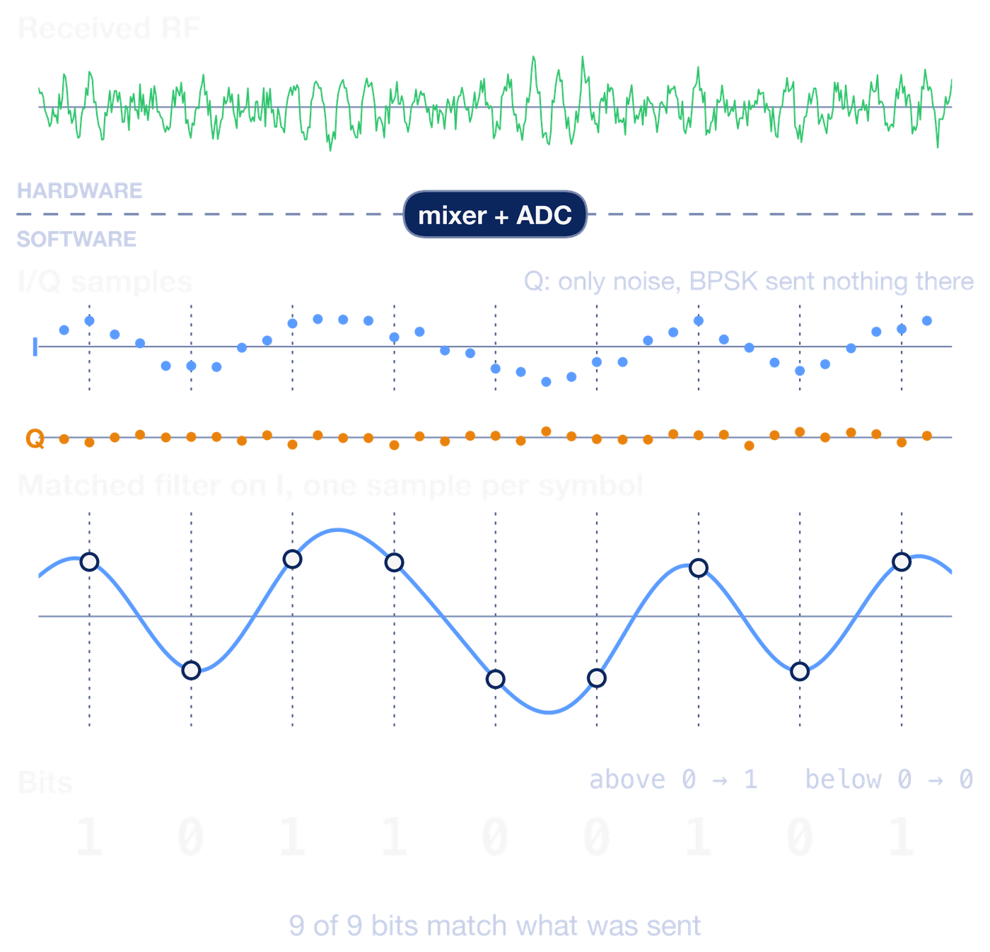
All nine bits come back. The samples land between 0.88 and 1.14 in size, close to ±1.
Why put half the filter at each end? It solves two separate problems.
The first is interference between symbols. Each pulse is wider than one symbol, so neighbouring pulses overlap. The two root-raised-cosine filters together form a raised-cosine pulse, which is exactly zero at every other symbol's sampling instant. The pulses still overlap in between, but at the moments the receiver looks, each symbol sees only itself. That is why the transmitted curve misses ±1 at the symbol centres while the received samples land back near it.
The second is noise. Noise enters after the transmitter, so only the receiver's filter can fight it. A filter shaped like the expected pulse, the matched filter, adds up the signal coherently while the noise partly cancels. It gives the best possible signal-to-noise ratio at the sampling instant.
Splitting the raised cosine into two root halves is what lets the receiver's filter do both jobs at once.
What Real Modems Add
The toy assumed the hard parts away. A real modem first has to synchronize: find the exact carrier frequency and phase, which drift, and the symbol timing. It needs framing, known headers that show where each frame starts and how it is coded. And it needs error correction, redundancy added at the transmitter so the receiver can repair bits that noise flips. The weather satellite walkthrough shows these steps on a real recording. All of them are still software working on I/Q samples, and that has a consequence for where the modem can live.
Why the Modem Can Run Anywhere
Nothing in that modem needs to sit next to the antenna, as long as the network between them is up to the job: enough bandwidth, accurate timing, and reliable transport. Given that, the modem needs the samples and a description of them: centre frequency, sample rate, number format. Without the description, a stream of numbers is meaningless. Three standards carry the description with the samples, each for a different job.
Recordings: SigMF
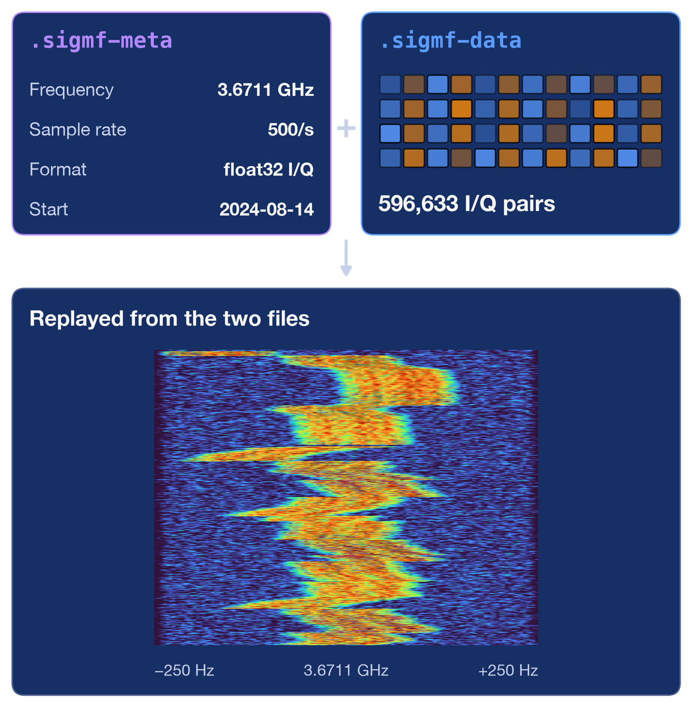
SigMF stores a recording as two files. The samples go in a .sigmf-data file, and the description goes in a small JSON file beside it, .sigmf-meta. Any tool that reads the pair knows what the numbers mean. A recording made at one site can be replayed into a different modem or analysis tool months later, with nothing to guess.
Live Streams: VITA-49
A recording is not enough for live operations. VITA-49 sends the samples and their description on one network stream. Data packets carry timestamped I/Q samples. Context packets carry the description and are repeated, so a receiver that joins late knows what it is looking at, and a retune is announced inside the stream itself.
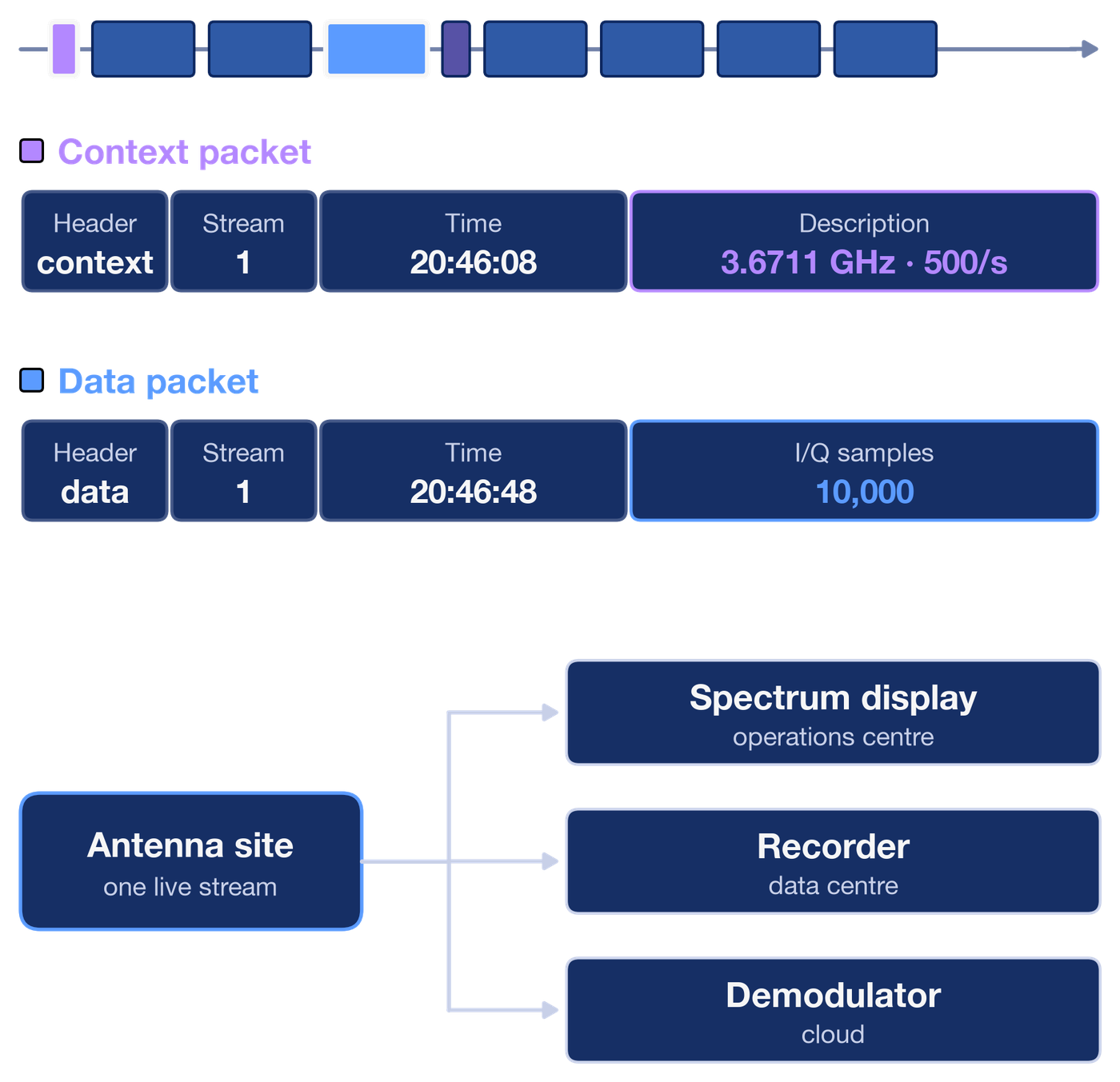
With the description travelling alongside the samples, the modem for our transponder can be a program in a data centre, and the same stream can feed a recorder and a spectrum monitor at once.
Interoperability: DIFI
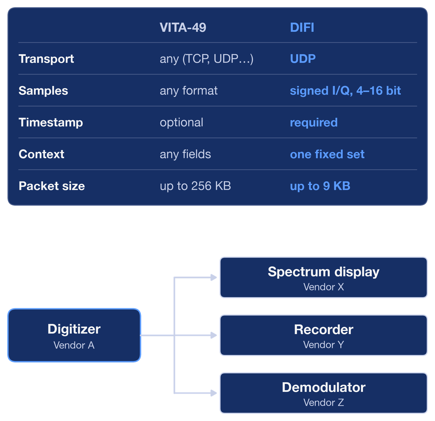
VITA-49 leaves many choices open: the transport, the sample format, which context fields to send. Two products can both comply and still not understand each other. DIFI (IEEE-ISTO Std 4900) is a strict profile of VITA-49 that makes those choices once. That enables interoperability between compliant implementations, so a digitizer from one vendor can feed a demodulator from another.
Hardware at the Edge, Software Everywhere Else
Follow one signal and the boundary is easy to find. The antenna gives a voltage. A mixer and an ADC turn it into I/Q samples. Everything after that is filters, decisions and bookkeeping on numbers.
That boundary is the idea behind a virtualized ground station. The antenna site keeps what has to touch the radio wave: the dish, the amplifiers, the frequency converters and the digitizer. A DIFI stream carries the samples over an ordinary network to modems that run as software, in a data centre or a cloud region. One antenna's stream can feed several modems and a recorder at once. Adding a carrier or a waveform becomes a software deployment rather than more dedicated equipment, and a SigMF recording lets anyone replay a problem after the fact.
Hardware still sets the limits. Amplifier noise, converter range and antenna gain decide how clean the samples are, and nothing downstream can add back what they lose. The network becomes part of the chain too: streaming our transponder at 40 million complex samples a second, with 16 bits each for I and Q, takes about 1.3 Gbps. That stream needs a network with the capacity to carry it, timestamps accurate enough to keep samples in order and aligned, and transport that doesn't drop packets. Where the network can't provide those, the modem stays close to the antenna.
How clean those samples are also decides how much the link can carry, and that changes with the weather. That is the subject of Why Satellite Capacity Isn't Fixed.