Decoding a weather satellite, from raw radio to finished image

Right now, a satellite about 820 km overhead is photographing the Earth and broadcasting the pictures straight down, in the open, on a band anyone can tune. The signal is faint and the spacecraft is fast, but catching it needs no dish and no tracking mount: a simple wire antenna and a consumer software-defined radio will pull a live image of the planet out of the sky in the few minutes it is in view. This post does exactly that, once, end to end.

The spacecraft are the METEOR-M series, Russian polar-orbiting weather satellites that image the Earth on every pass and broadcast it as LRPT (Low-Rate Picture Transmission) on the 137 MHz band. The pass here is METEOR-M2-3 (NORAD 57166), captured over Vancouver on 11 June 2026, followed through the whole receive chain: the antenna, the link geometry, the raw radio, the demodulation that turns samples into bits, and the decoded image. One thread ties the stages together: at each step the physics makes a prediction and the recording checks it. The antenna model predicts a gain null straight overhead; the orbit model predicts the exact Doppler curve. When each measurement lands on its prediction, that agreement is how you know the chain is working.

The Ground Station

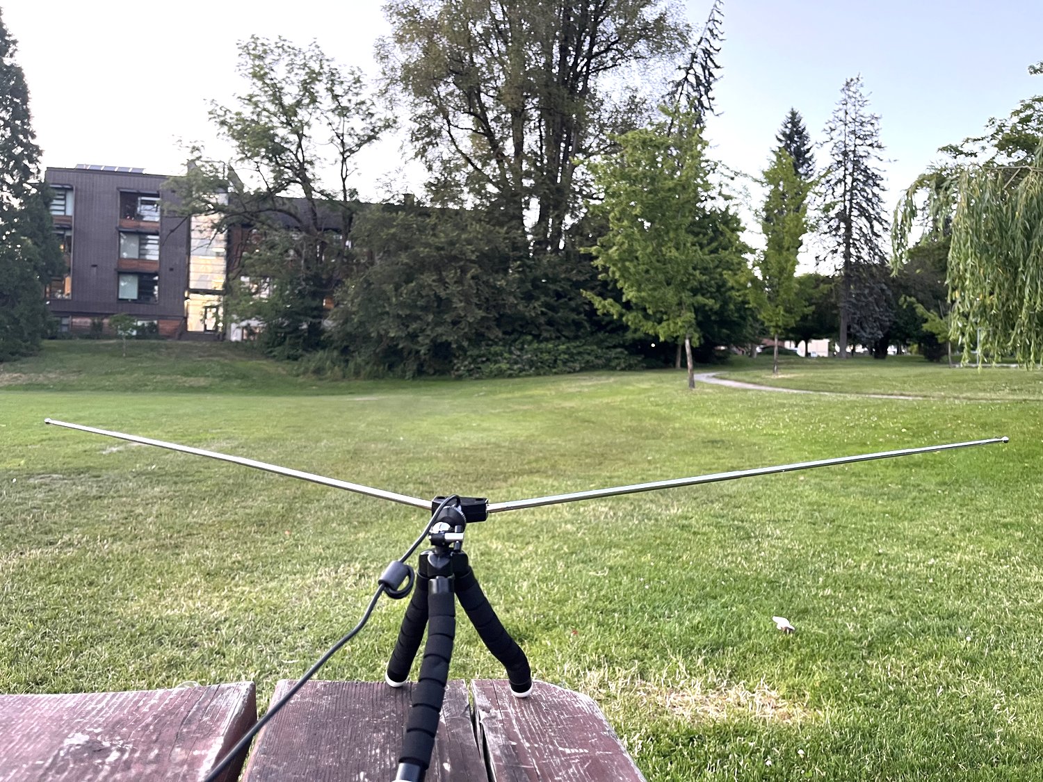
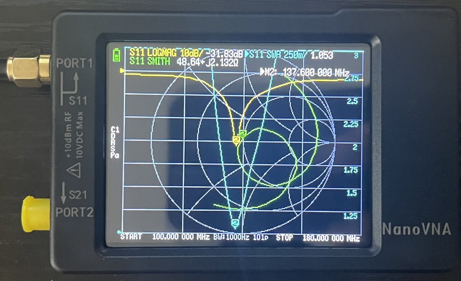
The ground station is three compact parts in a chain. The antenna is a horizontal V-dipole: two ~52 cm elements (a quarter wavelength at 137 MHz) set at roughly a 120° included angle. Its output passes through a SAWbird+ NOAA LNA, a 137 MHz SAW band-pass filter with an integrated low-noise amplifier mounted right at the antenna, which lifts the faint signal and rejects out-of-band interference ahead of the cable run. That feeds an RTL-SDR USB receiver, which digitises the band and streams raw IQ samples to a laptop. Before the pass the antenna's match is checked on a nanoVNA and the element lengths trimmed until it is resonant on the 137.9 MHz downlink. None of it is exotic, but each part has a specific job and the order matters.

Checking the antenna match

Three choices make a V-dipole work for polar satellites. Splayed into a shallow ~120° V: bending a straight dipole into a V broadens its azimuth pattern and fills the deep nulls a straight dipole has off its tips, so the satellite stays in a usable lobe across the whole arc, not just at broadside. Horizontal, about 1 m up (roughly half a wavelength at 137 MHz): the ground acts as a mirror, and the direct and reflected waves combine into lobes tilted up toward the mid and high elevations where a pass spends most of its time. Aligned north-south: polar satellites cross the sky roughly N-S, so laying the antenna along that line keeps them in its strong broadside for the whole pass.

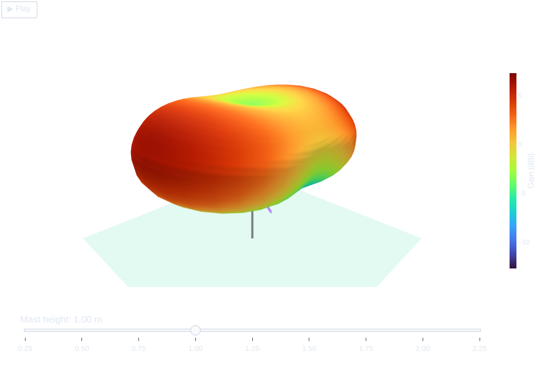
That half-wave height is a deliberate trade: it buys those upward lobes, but at exactly that height a null opens straight overhead, so a satellite at its closest, directly above, sits in the antenna's weakest direction. You can watch this in the model below: drag the height slider up from 0.25 m and the beam first points at the zenith, then tilts and splits toward the horizon until, right around half a wavelength (~1.1 m), the overhead null forms. That predicted null is the first thing the recording will let us test.

The Satellite Pass

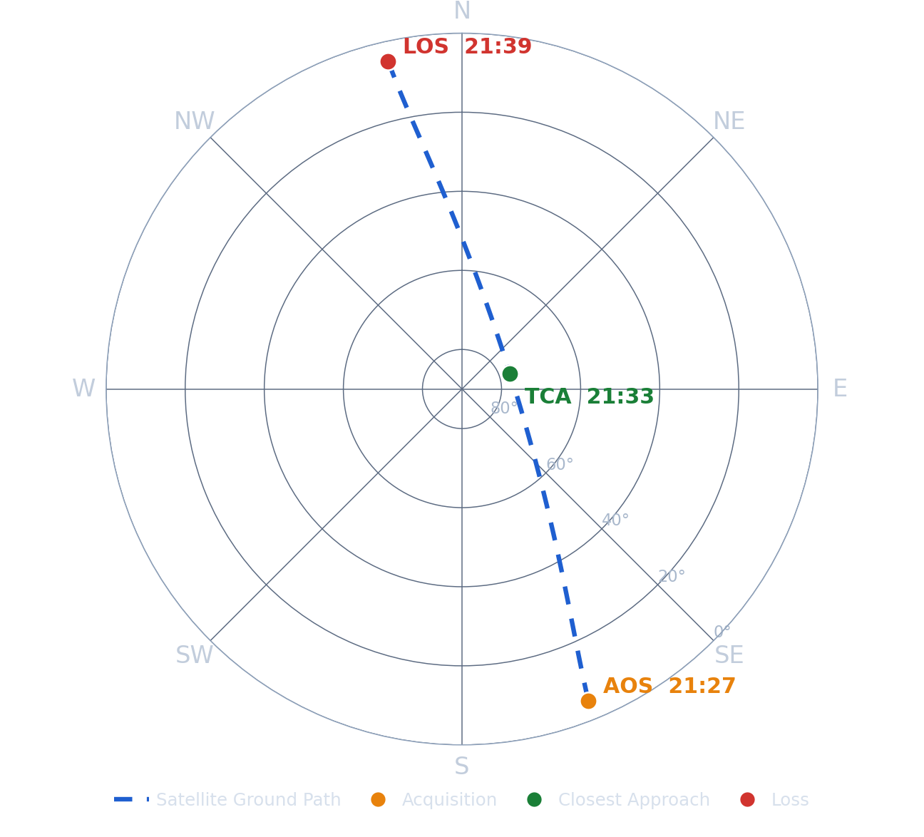
Here is the pass this recording captured. On 11 June 2026, METEOR-M2-3 made an ascending (south → north) pass over Vancouver, BC (~49°N, ~123°W), climbing to a near-overhead 77°. The sky-view below is computed from the TLE and drawn looking straight up: centre is the zenith, the rim is the horizon, the dashed line is the track. It rose in the SSE (21:27 local), peaked almost overhead (21:33), and set in the NNW (21:39). To receive it well you point the V's opening along the track (toward about 158°, SSE) with the elements across it, so the broadside faces the low rise and set points where the link is weakest. That is the orientation flown in the 3-D view next.

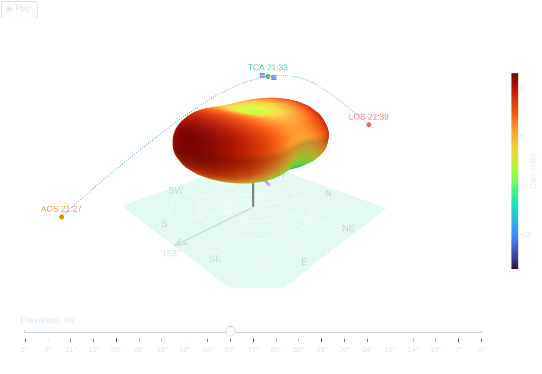
The same pass flown through the antenna's 3-D pattern, also computed from the TLE. The warm dome is antenna gain; the floor carries a compass and elevation rings aligned to the real bearings, with an arrow toward the acquisition azimuth and a live read-out of the satellite's true slant range (~2,300 km on the horizon, ~820 km overhead). Watch it tuck in close right overhead at closest approach, passing through the dome's weak zenith region exactly as the height sweep predicted. Drag to rotate; it pauses while you do.

The Signal

Now the radio. The receiver captured this pass as raw IQ samples: the antenna voltage shifted down near 0 Hz and sampled. From that one recording, three views tell the story: what the raw signal looks like, how its strength rose and fell, and how its geometry and Doppler shift line up with prediction.

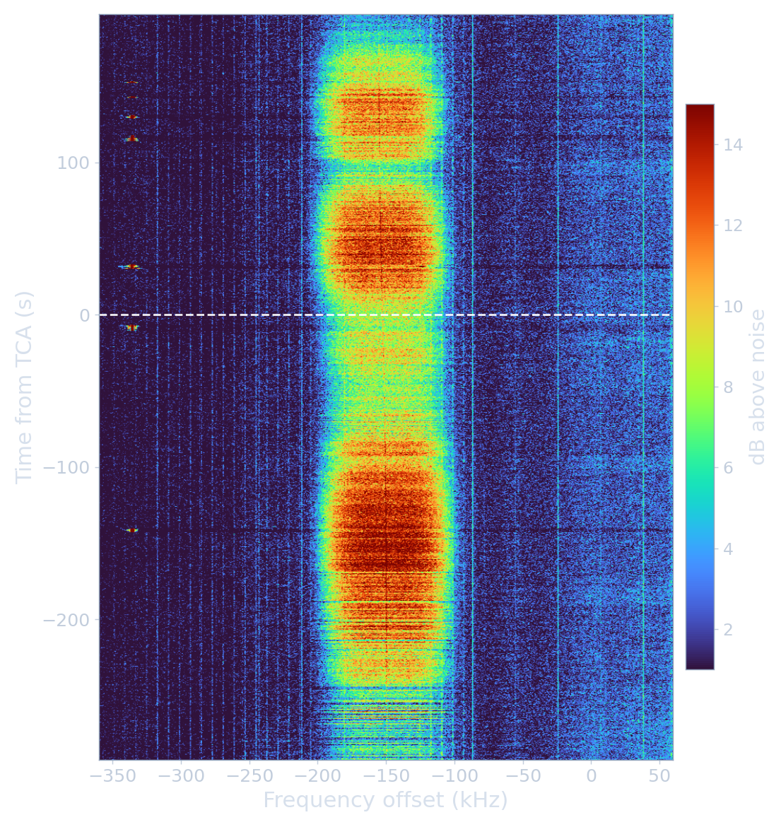
Below is the recording as a waterfall, with time running upward, frequency across, and brightness standing in for power. The broad band about 140 kHz wide near −150 kHz is METEOR-M2-3's LRPT signal, and time is referenced to closest approach (TCA = 0, the dashed line). The signal strengthens as the satellite climbs, fades noticeably around TCA as it passes nearly overhead through the antenna's weak zenith region, then brightens again before it sets. The faint vertical lines elsewhere are local interference and a stray carrier.

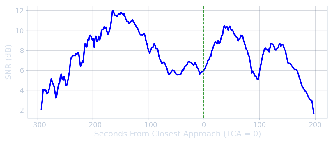
The signal-to-noise ratio over the pass shows when the satellite was workable, and it gives the first real chance to check the antenna model against data. The link stays usable for several minutes on this near-overhead capture (peak ~77°), wandering by a few dB as the satellite moves through the antenna's lobes and the geometry shifts. The most telling feature is the dip near closest approach, which falls right where the model places the antenna's weak overhead region. A measured fade is never purely a pattern effect, since polarization rotation through the ionosphere and ground multipath ride along with it, and METEOR-M2-3's own partially-deployed transmit antenna is known to wander the downlink polarization through a pass, so this is not a clean one-to-one match. But the dip landing where the predicted null sits, just as range is shortest and the signal should be strongest, is good evidence the overhead null is the main thing behind it.

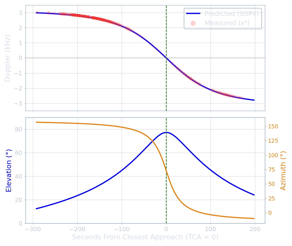
The Doppler shift is the second prediction the recording checks, and the figure below lays it over the geometry on one time axis. In the top panel, the carrier runs high on approach, slides through the true frequency at closest approach, and falls low as the satellite recedes, following $f_d = -\dfrac{\dot r}{c}\, f_0$, where $\dot r$ is the range-rate, $c$ the speed of light, and $f_0$ the carrier. Its slope is steepest right at the elevation peak (the dashed TCA line), where the satellite sweeps across the sky fastest. The points measured from the data (a 4th-power carrier estimate, with marker opacity showing confidence) sit on the curve predicted by the SGP4 orbit model the whole way, which validates the orbit and confirms you are locked onto the right satellite. The lower panel shows elevation reaching 77° and the azimuth swinging quickly through as it crosses nearly overhead.

Demodulation

This is where the waveform becomes bits. The shape of the pipeline follows directly from how the signal is built, so it is worth a moment on what we are demodulating and why.

LRPT is digital: a ~5 W transmitter sending 72,000 symbols/s at two bits each, a 144 kbit/s stream of compressed imagery. The bits sit in the carrier's phase, not its amplitude, because the satellite's amplifier runs saturated and nonlinear and would mangle any amplitude-bearing scheme like QAM; four phases 90° apart give two bits per symbol, which is QPSK. The offset in OQPSK takes that one step further: plain QPSK lets both bits flip at once, a 180° jump through the origin where the envelope drops to zero and the saturated amplifier turns the dip into spectral splatter. Offsetting one bit stream by half a symbol caps the phase step at 90°, keeps the path off the origin, and holds the envelope nearly constant. The price is the half-symbol stagger the receiver undoes at the end.

Each stage below has one job, and the figure shows the constellation tighten from a fuzzy blob into four clean clusters as they are applied in turn.

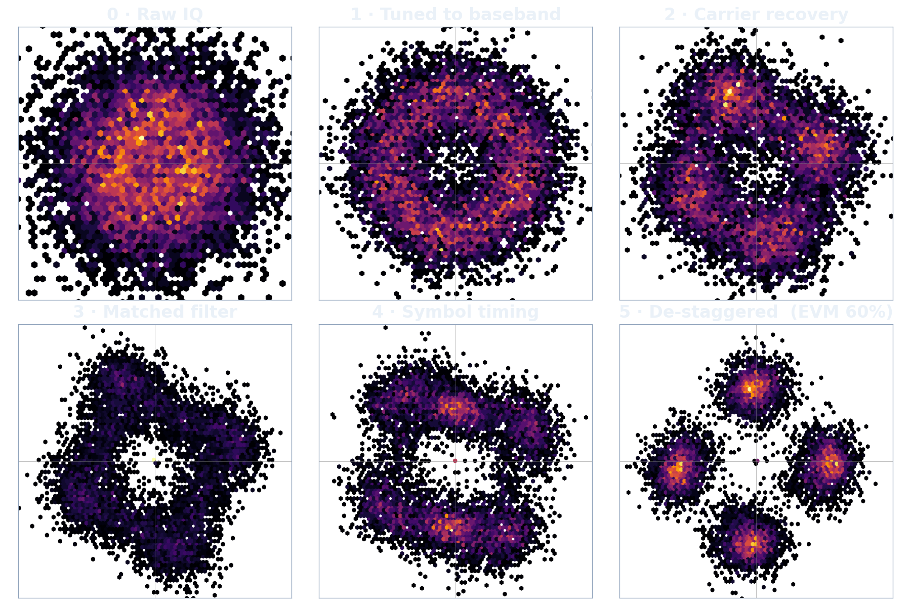
Tune and filter. The recording arrives with the LRPT band offset (near −150 kHz in the captured window) and a slowly drifting Doppler on top. This step mixes the band down to 0 Hz, low-pass filters to the signal's ~140 kHz, and resamples to four samples per symbol. That discards the interference, the stray carrier, and out-of-band noise, lifting the effective SNR; the information itself is untouched. In the figure the raw blob (0) becomes a ring (1): a residual frequency offset is still rotating the constellation, turning each successive symbol a little further than the last, so the four states smear into a continuous ring.

Carrier recovery. Removing that rotation is harder than it looks, because QPSK is suppressed-carrier: the modulation is balanced, so there is no leftover tone to lock onto, and the data keeps jumping the phase among four states. The fix is to raise the signal to the 4th power. The four phases are 90° apart, so multiplying every phase by four collapses them all onto one angle, stripping the data and leaving a single tone at four times the residual carrier offset (the $4f_c$ in the figure). Measure that tone, divide by four, and you have the error to correct, de-spinning the ring back into four blobs (2). Two honest caveats: the 4th power amplifies noise, and it pins phase only modulo 90°, leaving the constellation's absolute orientation ambiguous by a quarter turn, which the frame synchroniser resolves later.

Matched filter. The transmitter shaped each symbol with a root-raised-cosine pulse; the receiver applies the matching one here, doing two jobs at once. As the matched filter to that pulse it maximises SNR at the sampling instant, and because two root-raised-cosines multiply into a full raised-cosine, it meets the Nyquist condition for zero inter-symbol interference, so neighbouring symbols do not bleed into the decision.

Symbol timing. The matched filter only helps if each symbol is sampled at the right instant, and the receiver's clock is not aligned to the satellite's symbol clock. We recover the offset with the Oerder–Meyr method: squaring the signal makes a tone appear at the symbol rate, and the phase of that tone tells you where the symbol centres fall. It estimates this once per 256-symbol block, then takes one sample per symbol at the recovered instants. Unlike the tracking loops most SDR demods use, it is feedforward: one measurement per block, no loop to converge. That suits a batch toolkit, and it works here because the symbol clock holds steady across each block. Once locked the clusters tighten (3 to 4); the OQPSK offset is still in place, so this is not yet a clean four points.

De-stagger and slice. The last step undoes the half-symbol offset OQPSK added at the transmitter, realigning I and Q so both halves of each symbol line up again. The signal then reads as ordinary QPSK, the four clusters appear, and slicing is just asking which quadrant each sample fell in: two bits per symbol (5). This is where the spectral cleanliness OQPSK bought on the satellite gets paid back.

One last point. Those final clusters are loose: the error-vector magnitude (how far each symbol lands from where it should) is around 60%, so symbol by symbol, many decisions are simply wrong. They survive because the symbols carry forward error correction, redundancy added at the satellite to repair exactly these errors. This stage-by-stage walk was here to show what each block does, not to be the production decoder; the actual image comes from running SatDump, an open-source satellite signal decoder, on the same raw IQ recording, which demodulates and error-corrects it into the picture below.

The Decoded Image

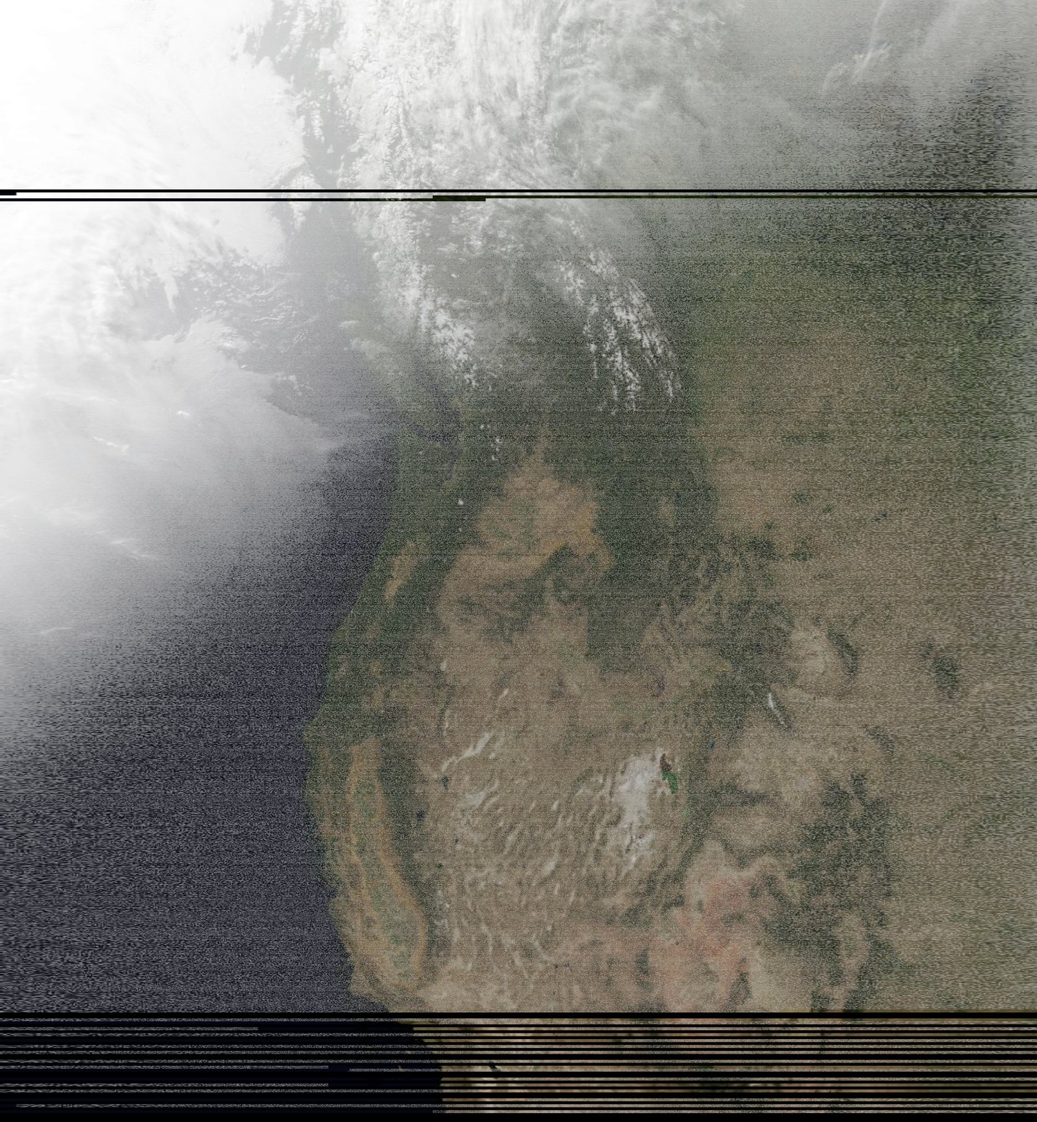
The payoff: the decoded MSU-MR image, produced by running the raw IQ recording through SatDump, which demodulates it and applies the error correction (frame sync, Viterbi, and Reed–Solomon). Each line was scanned by the satellite as it flew over and is stacked here in order, north up. It is the US West Coast: the Pacific on the left, the coastline down the middle, and the dry interior to the right. The ocean reads near-black because water reflects almost nothing in these channels, not because of the lighting; the land is brighter because it reflects more. The capture itself was at dusk with the sun low, so the whole scene is dim and low-contrast.

The black bands near the top and across the bottom are scan lines SatDump could not recover, lost at the start and end of the pass where the satellite sat low on the horizon at long range and the signal was weakest, exactly where the signal-to-noise trace bottomed out. The overhead null shows in that trace too, but it only dipped the link rather than breaking it, which is why the middle of the image holds together.

Lessons Learned

Getting one clean pass took several tries, and nearly every fix was about operating the chain better, not adding hardware. The LNA already sets the system's sensitivity at the antenna, so the SDR gain should run near its minimum; turning it up only clips the ADC, and one pass was lost when a strong nearby emitter at high gain saturated the front end. Geometry matters as much: a near-overhead pass drops the satellite into the antenna's zenith null at closest approach, so one peaking around 50 to 70 degrees works better. At a noisy, elevated site, recording at a narrower bandwidth (1.024 rather than 2.048 MHz) pushes out-of-band emitters out of the window, and a quick nanoVNA check confirms the dipole is resonant across 137 to 138 MHz. Finally, set up and verify ten minutes before acquisition and then keep your hands off, since most losses came from reacting mid-pass.

Closing the Loop

From a wire antenna to a finished image, the pass held together because every stage agreed with the physics that predicted it. The antenna model called for a gain null straight overhead, and the signal-to-noise trace dipped there on cue. The orbit model drew a Doppler curve before the satellite had even risen, and the measured carrier tracked it through closest approach and out the other side. The demodulator recovered a clean QPSK constellation from a faint, moving source, and the decoder turned those symbols into the swath above.

None of these steps is remarkable on its own. What makes the chain trustworthy is that each measurement landed where its model said it would, so by the time the image appears there is little left to doubt: it is not a lucky capture but the expected output of a system whose every link was checked against first principles. That is the real payoff of working through the chain stage by stage rather than treating the decoder as a black box. And because the whole walkthrough is driven by just a TLE, a ground location, and one recording, the same process repeats for the next pass, and the next satellite, with nothing more exotic than patience and a clear view of the sky.